1Computer Science Brown University Providence, RI 02912, USA;
e-mail: ldp@cs.brown.edu;
2Institute for Protein Research, Pushchino 142292, Russia;
e-mail: misha@imb.imb.ac.ru
+Corresponding author
Keywords: genomic DNA sequences, yeast genome, GC-content, hidden Markov models, chromosome segmentation
Introduction
Developed initially for speech recognition [Rabiner, 1989], hidden Markov models (HMM) are now widely used in computational molecular biology. The usual applications of HMMs include multiple alignment and functional classification of proteins [Krogh et al., 1994], prediction of protein folding [Di Francesco et al., 1997], recognition of genes in bacterial and human [Burge & Karlin, 1997, Kulp et al., 1996, Henderson et al., 1997] genomes, analysis and prediction of DNA functional sites [Crowley et al., 1997], and identification of nucleosomal DNA periodical patterns [Baldi et al., 1996].
However, the first application of HMMs to the analysis of genetic data, done by Churchill [Churchill, 1989, Churchill, 1992], was to analyze compositional heterogeneity of natural DNA sequences. Despite the importance of this pioneering work, a number of questions has remained unresolved. First, computational problems precluded analysis of long sequences, and allowed only the use of models with a small number of states (two or three). Second, no analysis of consistency of the generated segmentation or statistical confidence of a model choice was undertaken, and the features of the model parameter space were not analyzed. Finally, new data became available recently – in particular some complete genomes and chromosomes which provide an interesting subject of the analysis.
The present work aims to fill some of these gaps and addresses general properties of HMMs in the domain of DNA sequences. We systematically investigate the computational aspects such as the structure of the parameter space, the model likelihood landscapes and robustness of the obtained data segmentation. The algorithms are applied both to natural and simulated DNA sequences.
The amount of G+C is variable and characteristic of individual DNA molecules. Because the two strands are complementary, it is sufficient to represent a DNA molecule by the sequence of bases on a single strand. In addition to this four letter representation, it is sometimes of interest to consider binary representations. In this paper we address strong-weak hydrogen bonding (GC-AT or S-W respectively) classification.
Statistical properties of genomic DNA sequences are not well understood even at the simplest level of base composition. It is clearly non-uniform. In the l phage, the segments corresponding to early and late genes have different GC-AT composition [Churchill, 1989]. The shift of the GT-AC composition allows recognition of replication origins in bacteria [Lobry, 1996]. Recently acquired regions of bacterial genomes have unusual base composition [Medigue et al., 1991]. GC-rich segments often occur in regulatory regions of vertebrate genes, the GC-content of protein coding regions is higher than that of non-coding region in mammals and plants [Aissani et al., 1991].
The most popular theory is that the nuclear genomes of eukaryotes are composed of large segments (tens or hundreds of Kilobases, Kbp) which have fairly homogeneous G+C content within themselves and fall into one of a small number of distinct classes with different characteristic proportions of G+C [Bernardi, 1989]. These large regions, called isochores, are interspersed in some yet undetermined fashion throughout each chromosome. This kind of fundamental organization of DNA is likely to be related to a number of structural and functional properties of chromosomes, most of which are only conjectured at this time.
An alternative model is that changes in G+C contents are better described by smooth variations in parameters of a stochastic distribution, which could be modeled as a random walk with reflecting bounds [Fickett et al., 1992]. It means that, in fact, there are no long chunks of chromosomes with homogeneous distribution (isochores), but rather short ones, or no homogeneity at all. According to this model, there are states with little difference in distribution among which system chooses at any point, thus large variations are achievable only through little subsequent changes.
Results
Yeast Saccharomyce cerevisiae chromosomes I (230 Kbp) and V I (270 Kbp) [Goffeau et al., 1996] were downloaded from Stanford’s DNA Sequence and Technology Center. This sequence contains 230200 bp with 69832 (30.34%) of A, 44642 (19.39%) of C, 45762 (19.88%) of G and 69964 (30.39%) of T. AT-CG ratio is 39.3%-60.7% and AG/CT ratio is 50.22%-49.78%. Since we are only concerned here with GC contents, sequences were converted into binary format (1 for a strong bond, 0 for a weak bond), so what we model is a fraction of strong bonds along DNA sequence.
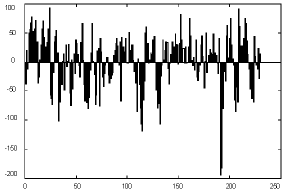
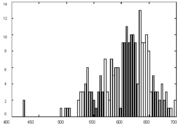
Figure 1 presents variations in C + G contents for Yeast chromosome I within a window of 1000 base pairs. It is quite evident that there are parts of a sequence with rather different statistics, but the question is – how many different categories should we introduce for statistically optimal description, in other words – how many states would the best model have and where would the segment borders be. The histogram of G+C content variation (Figure 1) suggests a multimodal distribution (mixture of 3-4 Gaussians) as well.
Figure 2 presents the segmentation of Yeast CH I by the best models in the order range two to six. Numbers on the left indicate the order of the model and the probability of observing a strong bond, corresponding to each state. The lower stripe corresponds to the two-state HMM segmentation, the upper to the six-state HMM segmentation. The segmentation picture significantly evolves when we go from order 2 to 3 and up to order 4 HMM. Although as we further increase the number of states there is no significant change in the segmentation. The fifth state with value 0.043 is only visited twice very briefly along the whole sequence of 230 Kbp. As a matter of fact we only stay at this state 0.06% of the length, while both states :29 and :52 used approximately 3% each, state :44 for 24% and state :37 for remaining 69% of a hidden sequence length.
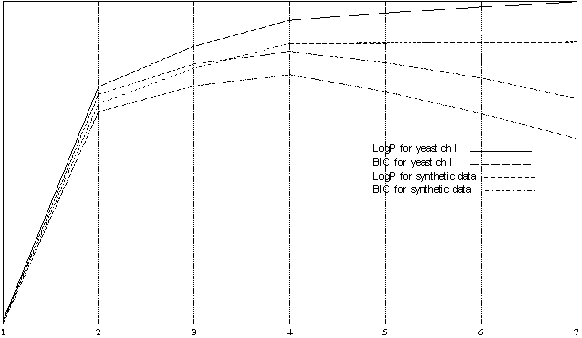
For comparison, in the optimal model of order four, the least used state still describes 3:5% of the length. This gives us an alternative criterion for deciding which order is the optimal for the description of a given sequence. We observe that in this application domain such a criterion agrees with Bayesian information criterion which is based on purely statistical considerations.
Figure 2 illustrates locations which are agreed upon by models of different orders as places of transition between two states. We have examined those locations and found that they often correspond to some biologically meaningful spots in DNA such as subtelomeric (terminal) regions. Note the difference in the usage of states to describe the distribution at different locations. Some fragments of DNA, for example from position 152228 to 189740 – almost 40 Kbp long – are well described by a uniform distribution, while others, for example location around 73469, are using all available states to describe the complexity of distribution. Comparison of compositional fragments of such information-rich regions can lead us to interesting results.
Experiments with yeast chromosome VI gave similar outcome and for brevity, we do not present these segmentation results here.
Figure 3 presents the comparison of the best models of different order using Log-likelihood and BIC for Yeast I and a synthetic data sample generated using the best four-state model for yeast CH I. The synthetic data clearly has ideal model of order four and all models with higher number of states do not add anything to the picture and usually have degenerate extra states which are never visited. We use this data for comparison to Yeast CH I and conclude that those likelihood profiles are very close, which gives us a additional proof that an HMM of order four is the best for Yeast Chromosome I. BIC for state four has a significantly higher value and provides us with a confident choice.
For Yeast CH VI models of order 3 and 4 have a very close value of BIC, but order 3 is slightly better. Remarkably, models for Yeast CH VI and CH I of order three (given below) use the same states – meaning that both chromosomes use the same fragments in the mosaic construction of DNA, which is natural since they belong to the same genome. We have also compared the distribution of segment lengths among Yeast CH I, Yeast CH VI, synthetic data and an equally long piece from the genome of E.coli, and found the distributions of segment lengths for two Yeast chromosomes to be very close to each other and significantly different from the other two samples of data.
|
|
|
|
| Figure 1. (Upper) GC content variations in Yeast Ch I; (Down) Histogram for GC content variations. |
|
|
| Figure 2. Segmentation of Yeast Ch I by HM models of different order. Numbers on the left indicate the order of the model and the probability of observing a strong bond, corresponding to each state. The lower stripe corresponds to the two-state HMM segmentation, the upper, to the six-state HMM segmentation. |
|
|
| Figure 3 the comparison of the best models of different order using Log-likelihood and BIC for Yeast I and a synthetic data sample generated using the best four-state model for yeast CH I. |
Discussion
Dividing genomes into compositionally homogeneous regions is important for a number of reasons. First, these segments have biological meaning (in particular, there is preliminary evidence that GC-rich segments almost always occur in intergenic regions). Second, it is well known that performance of many algorithms for functional mapping of genomic DNA sequences crucially depends on homogeneity of the sequences and it deteriorates when the sequences are not homogeneous. The compositional segmentation of genomes allows to use different sets of parameters fine-tuned for each composition and thus to improve performance (Burge and Karlin, 1997). Finally, this segmentation says something about the statistical properties of natural DNA, and in particular, assist in finding “foreign”, or recently aquired segments.
The obtained results demonstrate that HMMs are a useful and convenient tool for segmentation of genomic sequences into compositionally homogeneous segments. They provide a robust segmentation which does not depend on chromosome used to derive the model (of course, if it is not overtrained). All yeast models with 3 states are very similar, which is biologically plausible. Indeed, the chromosomes are not stable units, and multiple translocations that have been occurring in course of evolution lead to homogenization of global statistical properties. We plan to apply this techniques to analysis of other genomes, in particular those of bacteria (with the aim of searching for foreign segments) and human (with the aim of testing Bernardi’s isochore theory).
References
- Aissani, B. et al. (1991). The compositional properties of human genes. J. Mol. Evol. 32, 493-503.
- Baldi, P. et al. (1996). Naturally occuring nucleosome positioning signanls in human exons and introns. J. Mol. Biol. 263, 503-510.
- Bernardi, G. (1989). Isochore organization of the human genome. Annu. Rev. Genet. 23, 637-661.
- Burge, C. & Karlin, S. (1997). Prediction of complete gene structures in human genomic DNA. J. Mol. Biol. 268, 78-94.
- Churchill, G. (1989). Stochastic models for heterogeneous DNA sequences. Bull of Math Biol, 51, 79-94.
- Churchill, G. (1992). Hidden Markov chains and the analysis of genome structure. Computers Chem, 16, 107-115.
- Crowley, E. et al. (1997). A statistical model for locating regulatory regions in genomic DNA. J. Mol. Biol. 268, 8-14.
- Di Francesco, V. et al. (1997). Incorporating global information into secondary structure prediction with hidden Markov models of protein folds. ISMB, 5,. 100-103.
- Fickett, J. W. et al. (1992). Base compositional structure of genomes. Genomics, 3, 1056-1064.
- Goffeau, A. et al. (1996). Life with 6000 genes. Science, 274, 563-567.
- Henderson, J et al. (1997) Finding genes in DNA with a hidden Markov model. J. Comp. Biol. 4, 127-141
- Krogh, A. et al. (1994). Hidden Markov models in computational biology: Application to protein modeling. J. Mol. Biol. 235, 1501-1531.
- Kulp, D. et al. (1996). A generalized hidden Markov model for the recognition of human genes in DNA. ISMB, 4, 134-141.
- Lobry, J. (1996). Asymmetric substitution patterns in the two DNA strands of bacteria. Mol. Biol. Evol. 13, 660-665.
- Medigue, C. et al. (1991). Evidence for horizontal gene transfer in escherichia coli specitation. J. Mol. Biol. 222, 851-856.
- Rabiner, L. R. (1989). A tutorial on hidden Markov models and selected applications in speech recognition. Proceedings of the IEEE, 77, 257-286.


